Table Of Content
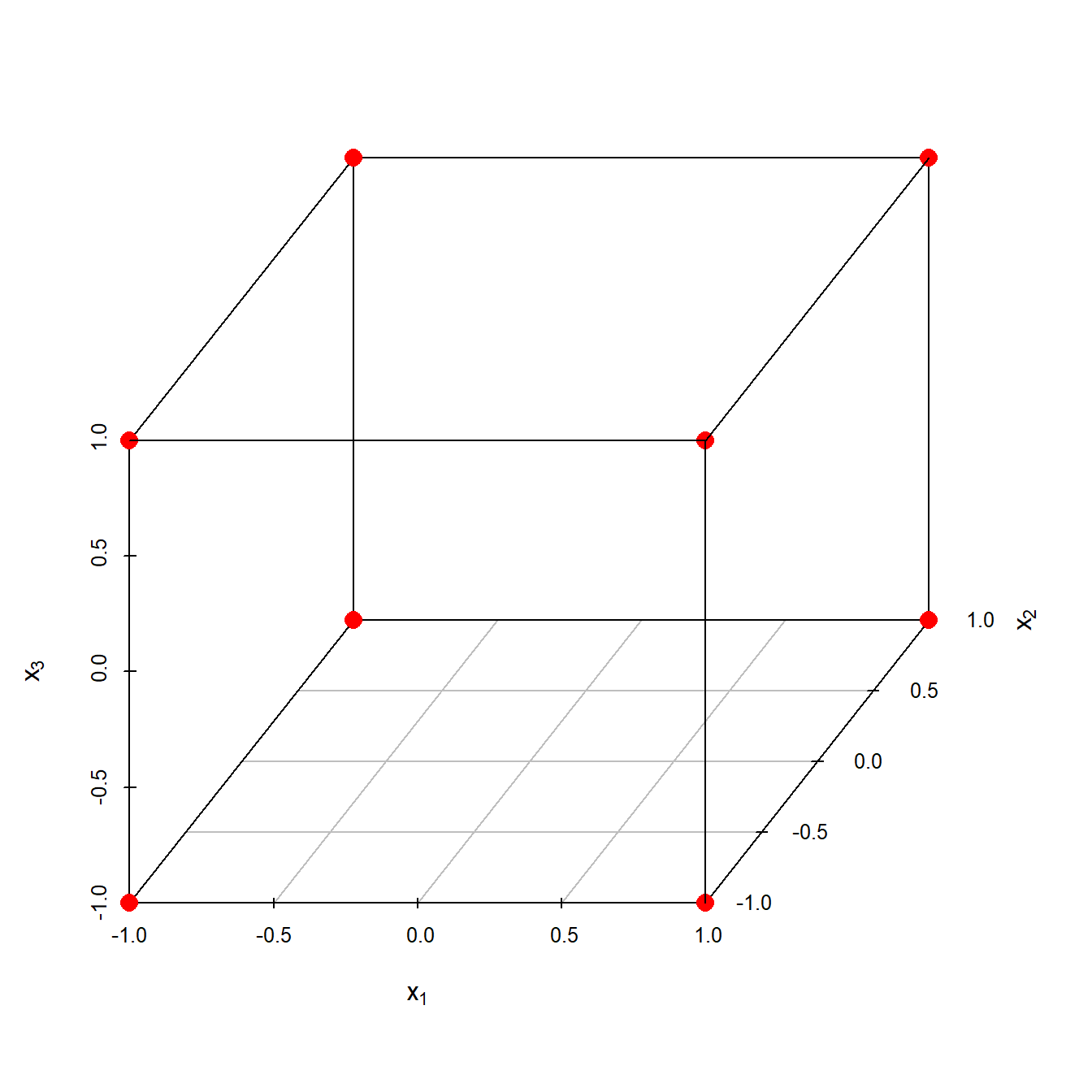
Factorial designs are therefore less attractive if a researcher wishes to consider more than two levels. As a further example, the effects of three input variables can be evaluated in eight experimental conditions shown as the corners of a cube. The interaction effects situation is the last outcome that can be detected using factorial design. From the example above, suppose you find that 20 year olds will suffer from seizures 10% of the time when given a 5 mg CureAll pill, while 20 year olds will suffer 25% of the time when given a 10 mg CureAll pill.
IV. Chapter 4: Psychological Measurement
Fertilizer B and 350 mL gave the second largest plant, and fertilizer B and 500 mL gave the second smallest plant. There is clearly an interaction due to the amount of water used and the fertilizer present. Perhaps each fertilizer is most effective with a certain amount of water.
Contrasts, main effects and interactions
The green bar for no-shoes is slightly smaller than the green bar for shoes. Instead of using tables to show the data, let’s use some bar graphs. The two contrast vectors for A depend only on the level of factor A. This can be seen by noting that the pattern of entries in each A column is the same as the pattern of the first component of "cell". (If necessary, sorting the table on A will show this.) Thus these two vectors belong to the main effect of A. Similarly, the two contrast vectors for B depend only on the level of factor B, namely the second component of "cell", so they belong to the main effect of B.
Factorial design optimized green reversed-phase high-performance liquid chromatography for simultaneous ... - ScienceDirect.com
Factorial design optimized green reversed-phase high-performance liquid chromatography for simultaneous ....
Posted: Thu, 09 Mar 2023 21:18:13 GMT [source]
& 4. Measure Performance to Find an Effect
All of the plots will pop-up on the screen and a text file of the results will be generated in the session file. Investigators may wish to adjust ICs to enhance their compatibility with other components. For instance, investigators might choose to reduce the burden of an IC by cutting sessions or contact times. This might reduce the meaning of the factor because it might make the IC unnecessarily ineffective or unrepresentative. This is less clear because the effect is smaller so it is harder to see. You can look at the red bars first and see that the red bar for no-shoes is slightly smaller than the red bar for shoes.
But when we fit a reduced model, now there is inherent replication and this pattern becomes apparent. All of the black dots are in fairly straight order except for perhaps the top two. If we look at these closer we can see that these are the BD and the BC terms, in addition to B, C, and D as our most important terms. Let's go back to Minitab and take out of our model the higher order interactions, (i.e. the 3-way and 4-way interactions), and produce this plot again (see below) just to see what we learn. We may also want contour plots of all pairs of our numeric factors.
Assigning Participants to Conditions
For example, it is possible that measuring participants’ moods before measuring their perceived health could affect their perceived health or that measuring their perceived health before their moods could affect their moods. So the order in which multiple dependent variables are measured becomes an issue. One approach is to measure them in the same order for all participants—usually with the most important one first so that it cannot be affected by measuring the others. Another approach is to counterbalance, or systematically vary, the order in which the dependent variables are measured. It would seem almost wasteful to measure a single dependent variable.
3.5. Identifying main effects and interactions
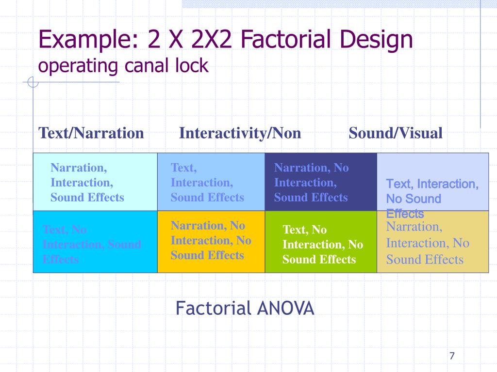
Notice that the number of possible conditions is the product of the numbers of levels. A 2 × 2 factorial design has four conditions, a 3 × 2 factorial design has six conditions, a 4 × 5 factorial design would have 20 conditions, and so on. Also notice that each number in the notation represents one factor, one independent variable. So by looking at how many numbers are in the notation, you can determine how many independent variables there are in the experiment. 2 x 2, 3 x 3, and 2 x 3 designs all have two numbers in the notation and therefore all have two independent variables. The numerical value of each of the numbers represents the number of levels of each independent variable.
While this algorithm is fairly straightforward, it is also quite tedious and is limited to 2n factorial designs. Thus, modern technology has allowed for this analysis to be done using statistical software programs through regression. When you look for the differences, it feels like you are doing something we would call “paying attention”. If you pay attention to the clock tower, you will see that the hands on the clock are different. We could give people 30 seconds to find as many differences as they can. So, our measure of performance, our dependent variable, could be the mean number of differences spotted.
Graphical Approaches to Finding a Model
It is important to keep in mind, however, that purely correlational approaches cannot unambiguously establish that one variable causes another. The best they can do is show patterns of relationships that are consistent with some causal interpretations and inconsistent with others. The example in Figure 5.15 shows a case in which it is probably a bit more straightforward to interpret both the main effects and the interaction.
Some questions to ask yourself are 1) can you identify the main effect of wearing shoes in the figure, and 2) can you identify the main effet of wearing hats in the figure. Both of these main effects can be seen in the figure, but they aren’t fully clear. To briefly add to the confusion, or perhaps to illustrate why these two concepts can be confusing, we will look at the eight possible outcomes that could occur in a 2x2 factorial experiment. For example, a shrimp aquaculture experiment[9] might have factors temperature at 25°C and 35°C, density at 80 or 160 shrimp/40 liters, and salinity at 10%, 25% and 40%.
So, the main effect of wearing shoes is to add 1 inch to a person’s height. Onwards, the minus (−) and plus (+) signs will indicate whether the factor is run at a low or high level, respectively. Frank Yates made significant contributions, particularly in the analysis of designs, by the Yates analysis.


No comments:
Post a Comment